Sunday, October 23, 2011

Numerical Analysis (Newton's Method)


Introduction

Newton's method is a technique for finding the root of a scalar-valued function f(x) of a single variable x. It has rapid convergence properties but requires that model information providing the derivative exists.

Background

Useful background for this topic includes:

References

Theory

Assumptions

Newton's method is based on the assumption that functions with continuous derivatives look like straight lines when you zoom in closely enough to the functions. This is demonstrated here.
We will assume that f(x) is a scalar-valued function of a single variable x and that f(x) has a continuous derivative f(1)(x) which we can compute.

Derivation

Suppose we have an approximation xa to a root r of f(x), that is, f(r) = 0. Figure 1 shows a function with a root and an approximation to that root.
Figure 1. A function f(x), a root r, and an approximation to that root xa.

Because f(x) has a continuous derivative, it follows that at any point on the curve of f(x), if we examine it closely enough, that it will look like a straight line. If this is the case, why not approximate the function at (xa, f(xa)) by a straight line which is tangent Txa to the curve at that point? This is shown in Figure 2.

Figure 2. The line tangent to the point (xa, f(xa)).

The formula for this line may be deduced quite easily: the linear polynomial f(1)(xa) ⋅ (x - xa) is zero at xa and has a slope of f(1)(xa), and therefore, if we add f(xa), it will be tangent to the given point on the curve, that is, the linear polynomial


is the tangent line. Because the tangent line is a good approximation to the function, it follows that the root of the tangent line should be a better approximation to the root than xa, and solving for the root of the tangent is straight-forward:

HOWTO

Problem

Given a function of one variable, f(x), find a value r (called a root) such that f(r) = 0.

Assumptions

We will assume that the function f(x) is continuous and has a continuous derivative.

Tools

We will use sampling, the derivative, and iteration. Information about the derivative is derived from the model. We use Taylor series for error analysis.

Initial Requirements

We have an initial approximation x0 of the root.
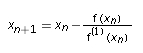
Iteration Process

Given the approximation xn, the next approximation xn + 1 is defined to be

Halting Conditions

There are three conditions which may cause the iteration process to halt:
  1. We halt if both of the following conditions are met:
    • The step between successive iterates is sufficiently small, |xn + 1 - xn| < εstep, and
    • The function evaluated at the point xn + 1 is sufficiently small, |f(xn + 1)| < εabs.
  2. If the derivative f(1)(xn) = 0, the iteration process fails (division-by-zero) and we halt.
  3. If we have iterated some maximum number of times, say N, and have not met Condition 1, we halt and indicate that a solution was not found.
If we halt due to Condition 1, we state that xn + 1 is our approximation to the root.
If we halt due to either Condition 2 or 3, we may either choose a different initial approximation x0, or state that a solution may not exist.

Error Analysis

Given that we are using Newton's method to approximate a root of the function f(x).
Suppose we have an approximation of the root xn which has an error of (r - xn). What is the error of the next approximationxn + 1 found after one iteration of Newton's method?
Suppose r is the actual root of f(x). Then from the Taylor series, we have that:

where ξ ∈ [rxn]. Note, however, that f(r) = 0, so if we set the left-hand side to zero and divide both sides by f(1)(xn), we get:


We can bring the first two terms to the left-hand side and multiple each side by -1. For the next step, I will group two of the terms on the terms on the left-hand side:


Note that the object in the parentheses on the left-hand side is, by definition, xn + 1 (after all, xn + 1 = xn - f(xn)/f(1)(xn) ), and thus we have:


But the left hand side is the error of xn + 1, and therefore we see that error is reduced by a scalar multiple of the square of the previous error.
To demonstrate this, let us find the root of f(x) = ex - 2 starting with x0 = 1. We note that the 1st and 2nd derivatives of f(x) are equal, so we will approximate ½ f(2)(ξ)/f(1)(xn) by ½. Table 1 shows the Newton iterates, their absolute errors, and the approximation of the error based on the square previous error.
Table 1. Newton iterates in finding a root of f(x) = ex - 2.
nxnerrn = ln(2) - xn½ errn - 12
01.0-3.069 ⋅ 10-1N/A
10.735758882342885-4.261 ⋅ 10-2-4.708 ⋅ 10-2
20.694042299918915-8.951 ⋅ 10-4-9.079 ⋅ 10-4
30.693147581059771-4.005 ⋅ 10-7-4.006 ⋅ 10-7
40.693147180560025-8.016 ⋅ 10-14-8.020 ⋅ 10-14
Note that the error at the nth step is very closely approximated by the error of the (n - 1)th step. Now, in reality, we do not know what the actual error is (otherwise, we wouldn't be using Newton's method, would we?) but this reassures us that, under reasonable conditions, Newton's method will converge very quickly.

Failure of Newton's Method

The above formula suggests that there are three situations where Newton's method may not converge quickly:
  1. Our approximation is far away from the actual root,
  2. The 2nd derivative is very large, or
  3. The derivative at xn is close to zero.

Examples

Example 1

As an example of Newton's method, suppose we wish to find a root of the function f(x) = cos(x) + 2 sin(x) + x2. A closed form solution for x does not exist so we must use a numerical technique. We will use x0 = 0 as our initial approximation. We will let the two values εstep = 0.001 and εabs = 0.001 and we will halt after a maximum of N = 100 iterations.
From calculus, we know that the derivative of the given function is f(1)(x) = -sin(x) + 2 cos(x) + 2x.
We will use four decimal digit arithmetic to find a solution and the resulting iteration is shown in Table 1.
Table 1. Newton's method applied to f(x) = cos(x) + 2 sin(x) + x2.
nxnxn + 1|f(xn + 1)||xn + 1 - xn|
00.0-0.50000.16880.5000
1-0.5000-0.63680.02050.1368
2-0.6368-0.65890.00080000.02210
3-0.6589-0.65980.00060.0009
Thus, with the last step, both halting conditions are met, and therefore, after four iterations, our approximation to the root is -0.6598 .

Questions

Question 1

Find a root of the function f(x) = e-x cos(x) starting with x0 = 1.3 . The terminating conditions are given by εabs = 1e-5 and εstep = 1e-5.
Answer: 1.57079632679490 after five iterations.

Question 2

Perform three steps of Newton's method for the function f(x) = x2 - 2 starting with x0 = 1. Use a calculator for the third step.
Answer: 3/2, 17/12, 577/408 ≈ 1.414215686274510

Applications to Engineering

Consider the circuit, consisting of a voltage source, a resistor, and a diode, shown in Figure 1.


Suppose we wish to find the current running through this circuit. To do so, we can use Kirchhoff's voltage law (KVL) which says that the sum of the voltages around a loop is zero. For this, we need the model of diode which states that the relationship between the current and the voltage across a diode is given by the equation


Solving this equation for the voltage v and using values IS = 8.3e-10 A, VT = 0.7 V, and n = 2, we get from KVL that

This equation cannot be solved exactly for the current with any of the tools available in an undergraduate program (it requires the use of the Lambert W function). Therefore we must resort to using numerical methods:
Defining the left hand side of the equation to be v(i), we have to solve v(i) = 0 for i, and we will continue iterating until εstep< 1e-10 and εabs < 1e-5.Table 1. Newton's method applied to v(i).
ninin + 1|v(in + 1)||in + 1 - in|
00.02.964283918e-100.07242.96e-10
12.964283918e-103.547336588e-101.81e-35.83e-11
23.547336588-103.562680160-101.17e-51.53e-12
33.562680160e-103.562690102e-102.63e-99.94e-16
Therefore, the current is approximately 3.562690102e-10 A.

Matlab

Finding a root of f(x) = cos(x):
eps_step = 1e-5;
eps_abs = 1e-5;
N = 100;
x = 0.2;

for i=1:N
    xn = x - cos(x)/( -sin(x) );

    if abs( x - xn ) < eps_step && abs( cos( xn ) ) < eps_abs
       break;
    elseif i == N
       error( 'Newton\'s method did not converge' );
    end

    x = xn;
end

xn
        
What happens if you start with smaller values of x? Why?

Maple

The following commands in Maple:
with( Student[Calculus1] ):
NewtonsMethod( cos(x), x = 0.5, output = plot, iterations = 5 );
produces the plot in Figure 1: 

For more help on Newton's method or on the Student[Calculus1] package, enter:

?NewtonsMethod
?Student , Calculus1

Numerical Analysis (The Bisection Method)


Introduction

The bisection method is simple, robust, and straight-forward: take an interval [ab] such that f(a) and f(b) have opposite signs, find the midpoint of [ab], and then decide whether the root lies on [a, (a + b)/2] or [(a + b)/2, b]. Repeat until the interval is sufficiently small.

Background

Useful background for this topic includes:

References


Theory


Intermediate Value Theorem (IVT)

Given a continuous real-valued function f(x) defined on an interval [ab], then if y is a point between the values of f(a) and f(b), then there exists a point r such that y = f(r).
As an example, consider the function f(x) = sin(x) defined on [1, 6]. The function is continuous on this interval, and the point 0.5 lies between the values of sin(1) ≈ 0.841 and sin(6) ≈ -0.279. Thus, there is at least one point r (there may be more) on the interval [1, 6] such that sin(r) = 0.5. In this case, r ≈ 2.61799. This is shown in Figure 1.
Figure 1. The IVT applied to sin(x) on [1, 6] with y = 0.5.


Using the IVT to Bound a Root


Suppose we have a function f(x) and an interval [ab] such that either the case that f(a) > 0 and f(b) < 0 or the case that f(a) < 0 and f(b) > 0, that is, f(a) and f(b) have opposite signs. Then, the value 0 lies between f(a) and f(b), and therefore, there must exist a point r on [ab] such that f(r) = 0.
We may refine our approximation to the root by dividing the interval into two: find the midpoint c = (a + b)/2. In any real world problem, it is very unlikely that f(c) = 0, however if we are that lucky, then we have found a root. More likely, if f(a) and f(c) have opposite signs, then a root must lie on the interval [ac]. The only other possibility is that f(c) and f(b) have opposite signs, and therefore the root must lie on the interval [cb].
We may repeat this process numerous times, each time halving the size of the interval.

Example

An example of bisecting is shown in Figure 2. With each step, the midpoint is shown in blue and the portion of the function which does not contain the root is shaded in grey. As the iteration continues, the interval on which the root lies gets smaller and smaller. The first two bisection points are 3 and 4.
Figure 2. The bisection method applied to sin(x) starting with the interval [1, 5].


HOWTO


Problem

Given a function of one variable, f(x), find a value r (called a root) such that f(r) = 0.

Assumptions

We will assume that the function f(x) is continuous.

Tools

We will use sampling, bracketing, and iteration.

Initial Requirements

We have an initial bound [ab] on the root, that is, f(a) and (b) have opposite signs.

Iteration Process

Given the interval [ab], define c = (a + b)/2. Then
  • if f(c) = 0 (unlikely in practice), then halt, as we have found a root,
  • if f(c) and f(a) have opposite signs, then a root must lie on [ac], so assign b = c,
  • else f(c) and f(b) must have opposite signs, and thus a root must lie on [cb], so assign a = c.

Halting Conditions

There are three conditions which may cause the iteration process to halt:
  1. As indicated, if f(c) = 0.
  2. We halt if both of the following conditions are met:
    • The width of the interval (after the assignment) is sufficiently small, that is b - a < εstep, and
    • The function evaluated at one of the end point |f(a)| or |f(b)| < εabs.
  3. If we have iterated some maximum number of times, say N, and have not met Condition 1, we halt and indicate that a solution was not found.
If we halt due to Condition 1, we state that c is our approximation to the root. If we halt according to Condition 2, we choose either a or b, depending on whether |f(a)| < |f(b)| or |f(a)| > |f(b)|, respectively.
If we halt due to Condition 3, then we indicate that a solution may not exist (the function may be discontinuous).

Error Analysis

Given that we an initial bound on the problem [ab], then the maximum error of using either a or b as our approximation ish = b − a. Because we halve the width of the interval with each iteration, the error is reduced by a factor of 2, and thus, the error after n iterations will be h/2n.
Therefore, thus, if εstep is fixed, then we may immediately know how many steps are required, after which we are assured that the absolute error is less than εstep. The inequality
h / 2n

may be solved for an integer value of n by finding:


For example, suppose that our initial interval is [0.7, 1.5]. If we have an εstep value of 1e-5, then we require a minimum of ⌈log2( 0.8/1e-5 )⌉ = 17 steps.

Examples

Example 1

Consider finding the root of f(x) = x2 - 3. Let εstep = 0.01, εabs = 0.01 and start with the interval [1, 2].
Table 1. Bisection method applied to f(x) = x2 - 3.
abf(a)f(b)c = (a + b)/2f(c)Updatenew b − a
1.02.0-2.01.01.5-0.75a = c0.5
1.52.0-0.751.01.750.062b = c0.25
1.51.75-0.750.06251.625-0.359a = c0.125
1.6251.75-0.35940.06251.6875-0.1523a = c0.0625
1.68751.75-0.15230.06251.7188-0.0457a = c0.0313
1.71881.75-0.04570.06251.73440.0081b = c0.0156
1.71988/td>1.7344-0.04570.00811.7266-0.0189a = c0.0078
Thus, with the seventh iteration, we note that the final interval, [1.7266, 1.7344], has a width less than 0.01 and |f(1.7344)| < 0.01, and therefore we chose b = 1.7344 to be our approximation of the root.

Example 2

Consider finding the root of f(x) = e-x(3.2 sin(x) - 0.5 cos(x)) on the interval [3, 4], this time with εstep = 0.001, εabs = 0.001.
Table 1. Bisection method applied to f(x) = e-x(3.2 sin(x) - 0.5 cos(x)).
abf(a)f(b)c = (a + b)/2f(c)Updatenew b − a
3.04.00.047127-0.0383723.5-0.019757b = c0.5
3.03.50.047127-0.0197573.250.0058479a = c0.25
3.253.50.0058479-0.0197573.375-0.0086808b = c0.125
3.253.3750.0058479-0.00868083.3125-0.0018773b = c0.0625
3.253.31250.0058479-0.00187733.28120.0018739a = c0.0313
3.28123.31250.0018739-0.00187733.2968-0.000024791b = c0.0156
3.28123.29680.0018739-0.0000247913.2890.00091736a = c0.0078
3.2893.29680.00091736-0.0000247913.29290.00044352a = c0.0039
3.29293.29680.00044352-0.0000247913.29480.00021466a = c0.002
3.29483.29680.00021466-0.0000247913.29580.000094077a = c0.001
3.29583.29680.000094077-0.0000247913.29630.000034799a = c0.0005
Thus, after the 11th iteration, we note that the final interval, [3.2958, 3.2968] has a width less than 0.001 and |f(3.2968)| < 0.001 and therefore we chose b = 3.2968 to be our approximation of the root.

Example 3

Apply the bisection method to f(x) = sin(x) starting with [1, 99], εstep = εabs = 0.00001, and comment.
After 24 iterations, we have the interval [40.84070158, 40.84070742] and sin(40.84070158) ≈ 0.0000028967. Note however that sin(x) has 31 roots on the interval [1, 99], however the bisection method neither suggests that more roots exist nor gives any suggestion as to where they may be.

Questions

Question 1

Approximate the root of f(x) = x3 - 3 with the bisection method starting with the interval [1, 2] and use εstep = 0.1 and εabs= 0.1 .
Answer: 1.4375

Question 2

Approximate the root of f(x) = x2 - 10 with the bisection method starting with the interval [3, 4] and use εstep = 0.1 and εabs= 0.1 .
Answer: 3.15625 (you need a few extra steps for εabs)

Applications to Engineering

To be completed.

Matlab

The bisection method in Matlab is quite straight-forward. Assume a file f.m with contents
function y = f(x)
   y = x.^3 - 2;
exists. Then:
>> format long
>> eps_abs = 1e-5;
>> eps_step = 1e-5;
>> a = 0.0;
>> b = 2.0;
>> while (b - a >= eps_step || ( abs( f(a) ) >= eps_abs && abs( f(b) )  >= eps_abs ) )
    c = (a + b)/2;
    if ( f(c) == 0 )
       break;
    elseif ( f(a)*f(c) < 0 )
       b = c;
    else
       a = c;
    end
end
>> [a b]
ans = 1.259918212890625  1.259925842285156
>> abs(f(a))
ans =    0.0000135103601622
>> abs(f(b))
ans =    0.0000228224229404

Thus, we would choose 1.259918212890625 as our approximation to the cube-root of 2, which has an actual value (to 16 digits) of 1.259921049894873.
An implementation of a function would be
function [ r ] = bisection( f, a, b, N, eps_step, eps_abs )
    % Check that that neither end-point is a root
    % and if f(a) and f(b) have the same sign, throw an exception.

    if ( f(a) == 0 )
 r = a;
 return;
    elseif ( f(b) == 0 )
 r = b;
 return;
    elseif ( f(a) * f(b) > 0 )
        error( 'f(a) and f(b) do not have opposite signs' );
    end

    % We will iterate N times and if a root was not
    % found after N iterations, an exception will be thrown.

    for k = 1:N
        % Find the mid-point
        c = (a + b)/2;

        % Check if we found a root or whether or not
        % we should continue with:
        %          [a, c] if f(a) and f(c) have opposite signs, or
        %          [c, b] if f(c) and f(b) have opposite signs.

        if ( f(c) == 0 )
            r = c;
            return;
        elseif ( f(c)*f(a) < 0 )
            b = c;
        else
            a = c;
        end

        % If |b - a| < eps_step, check whether or not
        %       |f(a)| < |f(b)| and |f(a)| < eps_abs and return 'a', or
        %       |f(b)| < eps_abs and return 'b'.

        if ( b - a < eps_step )
            if ( abs( f(a) ) < abs( f(b) ) && abs( f(a) ) < eps_abs )
                r = a;
                return;
            elseif ( abs( f(b) ) < eps_abs )
                r = b;
                return;
            end
        end
    end

    error( 'the method did not converge' );
end

Maple

The bisection method in Maple is quite straight-forward:
> epsilon[abs] := 1e-5:
> epsilon[step] := 1e-5:
> f := x -> x^3 - 2:
> a := 0.0:
> b := 2.0:
> while b - a >= epsilon[step] or ( abs( f(a) ) >= epsilon[abs] and abs( f(b) ) >= epsilon[abs] ) do
    c := (a + b)/2;

    if f(c) = 0 then
       break;
    elif f(a)*f(c) < 0 then
       b := c;
    else
       a := c;
    end if;
end do:
> [a, b];
                               [1.259918214, 1.259925843]
> abs( f(a) );
                                      0.000013505
> abs( f(b) );
                                      0.000022826
Thus, we would choose 1.259918214 as our approximation to the cube-root of 2, which has an actual value (to 10 digits) of 1.259921050.

==========================================

SOURCE: https://ece.uwaterloo.ca/~dwharder/NumericalAnalysis/10RootFinding/bisection/

Sunday, October 16, 2011

Curiosidade sobre a quantidade de energia que a Terra recebe do sol

A Terra recebe por volta de 800.000.000.000.000.000 watts de potência do sol (equivalente a 800.000.000.000.000.000 joules por segundo). 62,5% desta potência são imediatamente refletidos pelas nuvens, pelos oceanos, etc. Do restante, o que não é refletido:
  • 50.000.000.000.000 W são usados pelas plantas terrestres para fotossíntese;
  • 30.000.000.000.000.000 W aquecem o ar, produzindo ventos;
  • 200.000.000.000.000.000 W evaporam água;
  • 400.000.000.000.000 W são usados pelas plantas marinhas para fotossíntese;
  • 70.000.000.000.000.000 W aquecem a Terra.
Depois disso tudo, eu te pergunto... quantos watts de potência tem o seu aparelho de som mesmo :D ?

O sol está tão longe daqui que mesmo viajando na velocidade da luz, levaríamos mais de 8 minutos para chegar até ele. Apesar de tamanha distância, olha só a quantidade de energia que chega aqui no planeta... e detalhe, a atmosfera filtra mais da metade, e mesmo assim ainda há dias onde reclamamos de calor...

Realmente, o ser humano não é nada...


LU Decomposition Method

This is an interesting and straightforward explanation of LU Decomposition I've recently found on YouTube:


Part 1:


Part 2:


This and much more is available at the "numericmethodsguy" channel, you can follow it to be updated on his latest content.